
To begin with, let us discuss the nature of a digital signal. This can be thought of as values or numbers on some (at least implied) time grid.

An example is a digital audio signal such as one would find on a CD. These typically have the features described below.

A digital system has an input signal, similar to the ones we've discussed above, and an output signal. For interesting systems these two signals will differ in some way.

One element of a digital system is a gain, whose function is quite simple. Each input value is gained or scaled by this value. Note the input and output values in the example below.

Another digital system element is the unit delay. You EEs might think of this as a shift register. Either way, the point is that whatever is on its input at time n-1, is on it's output at time n. Note the example.

Generally speaking, feedback in a digital system cannot happen except through a delay, as shown below. What happens, is the output at time n-1, is fed back and summed to the next input value. So y(n) = x(n) + y(n-1). Note the example.

Now, clearly interesting systems will be combinations of these various elements, such as the simple one below where a couple of gains are combined with a feedback element (which is created from a unit delay).

Now we'll talk about ways to analyze a system such as this one.

Let's take a step back and talk more generally for a minute. A system has an input and an output and is modified by something between. In the sample domain (n), we call that something between the "impulse response" of the system. A process called "convolution" describes mathematically how that impulse response is applied to the input to get the ouput.
This is all presented by way of definition. But we will not really use this information for this module, or the other modules we discuss. Instead, we will talk about the z-domain (z). If you have run accross z-transforms before and they made you angry or terrified, close your eyes and take two deep breaths.
Feel better? Actually, the part of this that you need to know is no where near as difficult as engineering writers and professors have tried to make it. Stick with me and you'll know everything important very shortly, and without the anger or fear.
Suffice it to say that things we do in the sample (or time) domain can be transformed to the z-domain. We do this because certain things become easier to understand and to do in that domain. And, for our purposes, we never actually need to do z-transforms and their inverses, except in a very limited and simple sense.
The z-transform of the impulse response is called the "transfer function." You will get to know it well during this course, and it's much easier than you probably imagined. The transfer function relates the z-transform of the input to the z-transform of the output. And this relationship is now simpler - a product (multiply) rather than a convolution.

We will never need to take the z-transforms and inverse z-transforms of the inputs and outputs in this course. But what we will do is take the z-transform of the defining the system, and use that to very simply get the transfer function.
We don't use the transfer function for implementing digital systems. But they help us very much in analyzing them. I'll show you.
First, recall the equation that we used to describe our system above: y(n) = ax(n) + by(n-1). Refer now to the chart below. The z-tranform comes from this through a very simple rule.

Did you see how that worked? Basically, x(n-1) turns into X(z)z^-1. The scale factors stay the same. Now that we have this equation in terms of Y(z), we can use algebra to get the transfer function, H(z), which is defined as Y(z)/X(z).

Did you see how we got the transfer function in the last chart? If not, work through it, Google on it, let me know, or do something. You can definitely get it, but if it's stumping you let's address that sooner rather than later.
We are now ready to talk about how the transfer function can help us understand the stability of a system.
To begin, let us try an example as shown below.
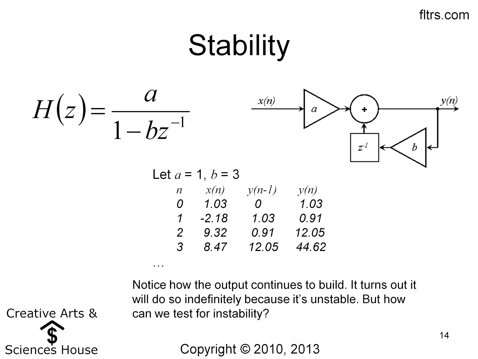
Now, we cannot tell from the output data above that the system is unstable, though we might be suspicious. But we can actually tell for sure even without computing the outputs, as we'll show below.

In our math unit we talked about the roots of polynomials. Transfer functions have (in general), both a numerator polynomial (upper portion) and a denominator polynomial (lower portion).
We call the roots of the numerator polynomial zeros of the system, and the roots of the denominator polynomial poles.

System theory tells us that a stable system must have poles with magnitudes strictly less than 1. Another way of saying this is that they much lie within the "unit circle," a circle in the complex plane with radius 1.
Our pole is 3, which is definitely greater than 1. As we suspected earlier, this system is unstable!

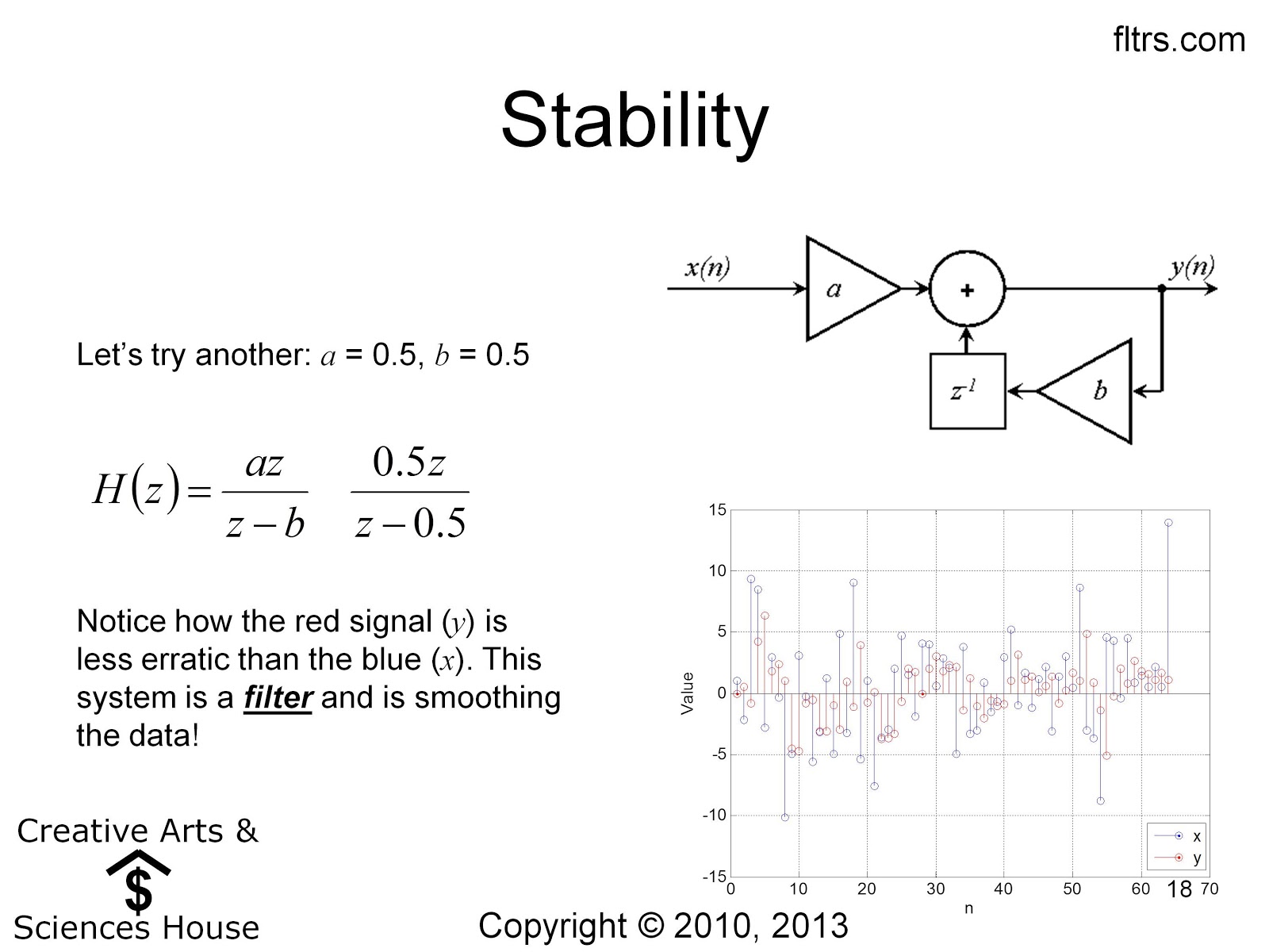
Let's try the case below:

We see above that the new pole is within the unit circle, so this is stable. But what does this system do?
We generated a random noise signal (blue) and passed it through this system. The output (red) is a little smoother. It turns out that we have created a simple filter.
Now let's try looking at this sort of thing in the opposite direction.

We can apply our z-transform relationship in reverse this time. Follow along.

Does it make sense? We've gone from a transfer function to a system equation. Now we can go from that to a block diagram. Note that there is more than one block diagram that will implement this equation, but that they are all mathematically the same (though might have some practical differences). Here we have drawn the "Direct Form I" diagram to implement this equation. More about that in a later unit.

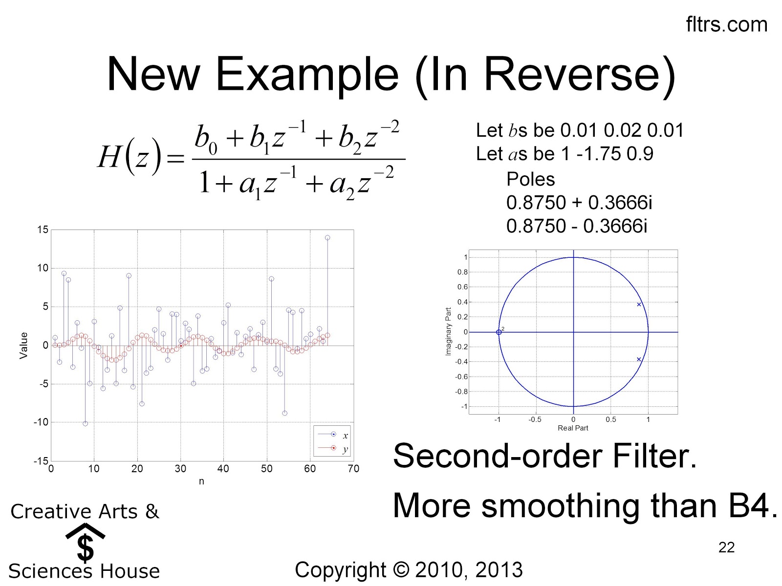
What does this system do? Well, again its coefficients make a difference as to its exact functionality. But again it's a filter (lowpass in fact) that smooths out the input even more than did our previous filter.
Notice that the poles are now complex, but that they do reside within the unit circle. The system is stable.
No comments:
Post a Comment