
This course follows my book, Digital Filters for Everyone. The book is not required for the course, but would be beneficial, especially if you are quite interested in this topic.

You are already familiar with filters, at least in the general case. There are water filters, air filters, even internet filters. Digital filters are filters in this sense, but are applied to electronic signals. And, in particular, to digital electronic signals. You'll see some examples below.

Filters are applied to electronic signals to reduce noise, to separate, enhance or attenuate various frequency components, or to perform some sort of mathematical operator to the signal.

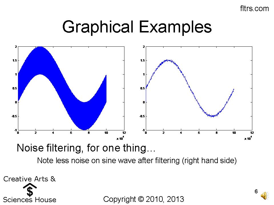
You might be familiar with a sine function, or a sine wave, as plotted below. The sine is a signal of a single frequency. However, the "fuzzy" sine at left is noisy. This means the signal has unwanted interference on it. We can use a filter to mitigate the interference, as shown in the plot at right. There are still some signs of interference, but it is much less after filtering.
The example above is a one-dimensional filter. But filtering can actually be done in two dimensions as well. The image at left is filtered to produce the image at right. Note that the left-hand image has a "salt and pepper" effect around the man's arm (as seen best in the zoomed image). Now notice two things about the filtered image at right: 1) the salt and pepper effect is less, and 2) the detail of the arm itself is actually blurrier (notice the watchband). This is typical of filtering. We very often trade off something less than desirable for something we need. The filter designer carefully considers these trade offs to determine the best compromise.

You might be familiar with Fourier series. But, if not, suffice it to say that a square wave can be created by summing numerous sine waves of the proper frequencies and amplitudes. Actually, it would take infinite sines to produce a proper square wave, but the square wave can be approximated by a handful of them. The formula for this is shown, along with a single sine at the fundamental frequency at left, and the result of three terms summed as shown at right.

The next couple of charts show the results of summing ten terms, and then fifty terms. Notice how the approximation to a square wave gets better and better as more terms are added.

Now, we can take our fifty term approximation and retrieve one of the sines from it by using a type of filter know as a bandpass. This filter passes only a small range of frequency and blocks all others. Depending upon where we set the passband of the this filter, we can retrieve whichever of the components we choose. (Note that all the filter terminology will make more sense in future courses. For now I just want to convince you that filters can be useful.)
Upper left is the fifty term square wave approximation. Upper right is the frequency response of the bandpass filter (don't worry about all the definitions for now). At bottom is the input signal (the fifty term approximation) superimposed with the output signal (the retrieved single frequency). We will discuss the output more on the next chart, but notice how it takes a while for the output signal to build up from zero. This is another characteristic of filters: one has to be careful to trust their outputs only after they've had sufficient time to "charge" or "settle."

Now at right we have the original 3rd component that went into the square wave approximation, and have zoomed into the output signal from our filter (after it has settled). You can still see some of the sine approximation (input signal) on the right-hand chart, though we've zoomed down to see the output signal. Notice that the output is a faithful representation of the original component.
NOTE: we would get this same output signal even for a true square wave input (that is, one not approximated by summing sines). Often filters are used to break signals into components.

There are few, if any, electronic devices without filters in them. And, these days, a large percentage of electronics actually include digital circuitry. The filters implemented in digital circuitry are, well, digital filters!

If you are interested in digital electronics, you might be interested in my book So You Want to be a 2-bit Digital Engineer. It covers the basics of digital electronics along with a tongue in cheek look at the engineering profession itself.
For now we'll just show a simple comparison. The left side of the chart below shows an analog signal and an analog filter, and the right side shows the digital versions of each.
Analog signals are continuous in both time and amplitude. Analog circuits are made up of components like resistors, capacitors and inductors.
Digital signals, on the other hand, are discrete (or quantized) in both time and amplitude. Digital circuits are made up of delays (z^-1), multiplies and sums. Some of this material will be found in my digital book or in other references on digital electronics. The structure of digital circuits themselves is covered in subsequent courses in this series.

Some standard filter types are shown graphically below. Note that the plots show magnitude on the y-axis (vertical), and frequency on the x-axis (horizontal). Where the magnitude line is high, the signal passes. Where it's low, the signal is attenuated. In the case of the shelf filter, all of the signals pass, but some pass with higher magnitude than others (that is, either some are attenuated, or some are emphasized depending upon the exact filter construction).
Filters are characterized by what frequencies they pass, low, high, band, etc. Note that the allpass filter is no joke. All frequencies pass equally, but the filter generally applies some phase effect to the signal. This is material for a later discussion. The nopass filter is, of course, a joke. At least until it happens to you sometime.

The next slide shows some standard filter terminology. The passband is the band of frequencies the filter passes, while the stopband is the band that it attenuates. Notice in this chart that there is a distinct "transition band," a slope between the passband and stopband. The previous chart showed the ideal case, with an abrupt transition. Unfortunately, this sort of thing is not realizable.
The filter parameter fc can mean critical frequency, center frequency, or corner frequency, depending upon context. For a lowpass filter, such as that shown, critical frequency and corner frequency both mean the same thing. Typically this is the point 3 dB below the passband level. But some filter types and some authors have different definitions. For a bandpass filter we would specify center frequency. Critical frequency works in this case as well; it is the more general term.

Now let's consider an example. You can read the text in the chart every bit as well as you could here, I assume, so I shall not repeat.

We've all worked this type of problem before. But, before today, you might not have know you were actually applying a digital filter. No point in trying to "teach" you anything you already know, so let's move on.

The implementation of the filter on the previous chart is shown below. We will study such block diagrams in more detail in a subsequent lesson. For now, just think of the z-1 blocks as delays. That is, whatever comes in the front of the filter on the first sample, will move into the first delay and be present on the next node at the next sample. In this way, a signal propagates through the filter one node at a time until a point where the first sample that entered is present at the last node, the sample before it is present at the node before, and so forth and so on. That is, at any point in time, this filter has the most recent seven samples of data at its various nodes. And each of these is multiplied by 1/7 and these products are all summed.
I know, it does seem like a lot of work to form a simple average. But this formalization of the average turns out to have a lot of power. We'll explore that over subsequent lessons. In the meantime, don't worry if the concept is a little fuzzy. We'll apply a defuzzification filter at a later time. :)

If we assume that our "signal" is the seven samples from our time trials, and that this signal is always 0 before and after our seven numbers, the filter output looks as seen below.
Before our number begin arriving in the filter, there are zeros on every node (this is an assumption, but one that is easy to force in practice). When our first time goes into the filter, the other nodes are all 0, so the output of the filter is just 1/7 of the first time. Do you see why?
This value is of no use to us, so we'll go on. The first sample moves one step deeper, and the second sample enters the filter. Now the output is 1/7 x the sum of the first two samples. Still not the number we want, but we're making progress, right?
And then some magic happens! Well, actually, it's not really magic. Rather, we repeat the same steps several times until the first sample appears at the last node. Now we have a fully loaded filter and the output is our average!
Then, if the filter keeps running, and if the signal has now gone to 0 as we assumed, the good samples shift away, the filter loads with 0s, and the output is no longer valid.
In an alternative universe, one in which we filter guys very often find ourselves, valid data could continue coming in to the filter, and its output would always be the average of the last seven samples. This type of filter goes by several names, including boxcar average, sliding average, or moving average.

In subsequent lessons we will discuss the meaning of the following plot in more detail, and even learn how to create it. For now, allow us to introduce our old friend the frequency response (or, more accurately, the magnitude response). This filter shows what happens in our seven sample averaging filter above, as a function of frequency. The frequency scale, for now, is normalized: 0 is 0 Hz, and 1 is one half of the sampling frequency, Fs, which is the so-called Nyquist frequency, and is the highest frequency our filter can affect.
We will also discuss dB scaled more later, but 20 dB is a factor of 10. This means that the lowest frequencies come through the average OK while higher frequencies tend to be attenuated by about a factor of ten. We'll learn later that a seven sample average is by no means a great lowpass filter. But it is a simple and reasonably effective one, and certainly has its uses.

The next two charts tell you more or less the subsequent lessons I plan to post. Although the material is already developed, it took me two days to type the notes included in this lesson. So be patient with me if you would. But I will work on getting another lesson out there soon. In the meantime, let me know your questions on this one and I'll do my best.


No comments:
Post a Comment