That was so nice; Thank You!

Many thanks to the reviewers of my book, Digital Filters for Everyone. If I am doing some things right, I appreciate you for letting everyone know. Bottom line: I am striving to make digital filters more accessible. Thanks to all who are helping me do that!

Digital Filter University - Course IV: Filter Theory

You may have been wondering when we'd get around to filter theory. Or maybe you paid attention in the first lecture and knew it would be now.

I couldn't have said it better if I'd ... oh yeah, I did say it myself. But once is enough.

Think back to the seven sample averging filter we discussed previously.

This filter can be drawn in standard filter notation as follows. Recall that the z^-1 element is a unit delay. This filter takes a seven-sample average of the most recent seven samples.

The averaging filter is an FIR or finite impulse response filter. The genera filter of this variety is shown below. Note that, generally speaking, this can have any number of delays and coefficients, and that the coefficients need not all be the same value.

Due to its utility in filter analysis, we define the impulse signal, which is valued 1 at one time (usually n=0), and 0 at all other times.

We use this impulse signal to get the impulse response of a filter. For an FIR filter, such as the average, the impulse response is just the list of coefficients, as you see here.

We are going to use the z-transform a an analysis tool for digital filters. In the sample domain, we have to 'convolve' the impulse response by the input to get the output. This is simple to do in HW but more difficult to do by hand. And, it doesn't teach us as much about the system as the 'frequency response,' which is the z-transform of the impulse response.

But don't worry. You might have run into z-transforms before and hated them. So did I. But I promise this time it will be simple and painless.

Recall that we can take our difference equation description, and change it to a z-transform description by applying a simple relationship as below.

Did you follow all that?

The transfer function is Y(z)/X(z). It tells us what we multiply the input by to get the output (in the z-domain, at least). The general (IIR) transfer function is shown. For FIR filters the denominator coefficients are all 0. (The funny upside down Vs, capital lambdas I guess, should have been ellipses (...). One day I might get around to updating the graphic.)

A step function is one that is zero up until a point, usually time 0, and then one forever after.

Like its very good friend the impulse function, the step function gives us insight into filter behavior.

Notice that it took the filter a while to "charge" up to the steady output of one. We learned something here about the "charge" time of the filter, and about how it will behave initially when hit with a new signal, or a large, long-lasting burst of energy even within a signal that it was already filtering.

We often plot filter responses on a dB scale. Decibels are defined below. This gives us a way to plot data with ranges that are otherwise too large to visualize.

We can get from the z-domain transfer function to the frequency response of a filter by substituting exp(i omega) for z, as shown below. This is a complex function. If we plot the magnitude (in dB, typically) as a function of frequency we have the magnitude response. We can also plot the phase, as shown below.

The phase above is actually linear, but "wrapped." If we were to "unwrap" it - remove the discontinuities at 180 degree intervals and attach the segments end to end - this one would be a nice linear function. Note how linear each segment appears. And there are ways to know, theoretically that it's perfectly linear.

When the phase is perfectly linear, it has a constant group delay. We see below that the group delay is the negative frequency derivative of the phase.

The Matlab code below shows how to create the filter response plots without using any fancy tools such as from the Signal Processing Toolbox. Similar commands could be used in other math tools. In my book I even show how to do it in Excel.

The arithmetic below shows how to use Euler's equations to get the frequency response of the averaging filter in terms of sines and cosines. You won't need to do all that by hand if you have access to a good math tool. And there are free ones out there.

Now let's think about this filter that showed up previously.

The frequency response for this filter, with the coefficients shown, is shown below. Note also how it smoothes the erratic noise signal (blue) to create the red output signal.



The phase response and group delay for this filter are shown. 

Recall the various types of filters. There are types not shown here, but this is most of the common ones.

If you use my book to design your digital filters, you will not need these, though their effects are embedded within my equations.

Many digital filters begin life as analog filters, and typically as a prototype analog lowpass filter. This prototype is then transformed, using one of the equations below, to have the desired critical frequency(ies) and to be of the desired type. After that it is transformed to digital.

Below are some of the standard forms for digital filters. Any of these can implement any filter type, depending upon the coefficients.



Digital Filter University - Course III: Digital Systems Theory

Our next topic is digital systems theory, upon which digital filter theory heavily relies.

To begin with, let us discuss the nature of a digital signal. This can be thought of as values or numbers on some (at least implied) time grid.



An example is a digital audio signal such as one would find on a CD. These typically have the features described below.

A digital system has an input signal, similar to the ones we've discussed above, and an output signal. For interesting systems these two signals will differ in some way.

One element of a digital system is a gain, whose function is quite simple. Each input value is gained or scaled by this value. Note the input and output values in the example below.

Another digital system element is the unit delay. You EEs might think of this as a shift register. Either way, the point is that whatever is on its input at time n-1, is on it's output at time n. Note the example.

Generally speaking, feedback in a digital system cannot happen except through a delay, as shown below. What happens, is the output at time n-1, is fed back and summed to the next input value. So y(n) = x(n) + y(n-1). Note the example.

Now, clearly interesting systems will be combinations of these various elements, such as the simple one below where a couple of gains are combined with a feedback element (which is created from a unit delay).

Now we'll talk about ways to analyze a system such as this one. 

Let's take a step back and talk more generally for a minute. A system has an input and an output and is modified by something between. In the sample domain (n), we call that something between the "impulse response" of the system. A process called "convolution" describes mathematically how that impulse response is applied to the input to get the ouput.

This is all presented by way of definition. But we will not really use this information for this module, or the other modules we discuss. Instead, we will talk about the z-domain (z). If you have run accross z-transforms before and they made you angry or terrified, close your eyes and take two deep breaths.

Feel better? Actually, the part of this that you need to know is no where near as difficult as engineering writers and professors have tried to make it. Stick with me and you'll know everything important very shortly, and without the anger or fear.

Suffice it to say that things we do in the sample (or time) domain can be transformed to the z-domain. We do this because certain things become easier to understand and to do in that domain. And, for our purposes, we never actually need to do z-transforms and their inverses, except in a very limited and simple sense.

The z-transform of the impulse response is called the "transfer function." You will get to know it well during this course, and it's much easier than you probably imagined. The transfer function relates the z-transform of the input to the z-transform of the output. And this relationship is now simpler - a product (multiply) rather than a convolution. 

We will never need to take the z-transforms and inverse z-transforms of the inputs and outputs in this course. But what we will do is take the z-transform of the defining the system, and use that to very simply get the transfer function.

We don't use the transfer function for implementing digital systems. But they help us very much in analyzing them. I'll show you.

First, recall the equation that we used to describe our system above: y(n) = ax(n) + by(n-1). Refer now to the chart below. The z-tranform comes from this through a very simple rule.  

Did you see how that worked? Basically, x(n-1) turns into X(z)z^-1. The scale factors stay the same. Now that we have this equation in terms of Y(z), we can use algebra to get the transfer function, H(z), which is defined as Y(z)/X(z).

Did you see how we got the transfer function in the last chart? If not, work through it, Google on it, let me know, or do something. You can definitely get it, but if it's stumping you let's address that sooner rather than later.

We are now ready to talk about how the transfer function can help us understand the stability of a system.

To begin, let us try an example as shown below. 

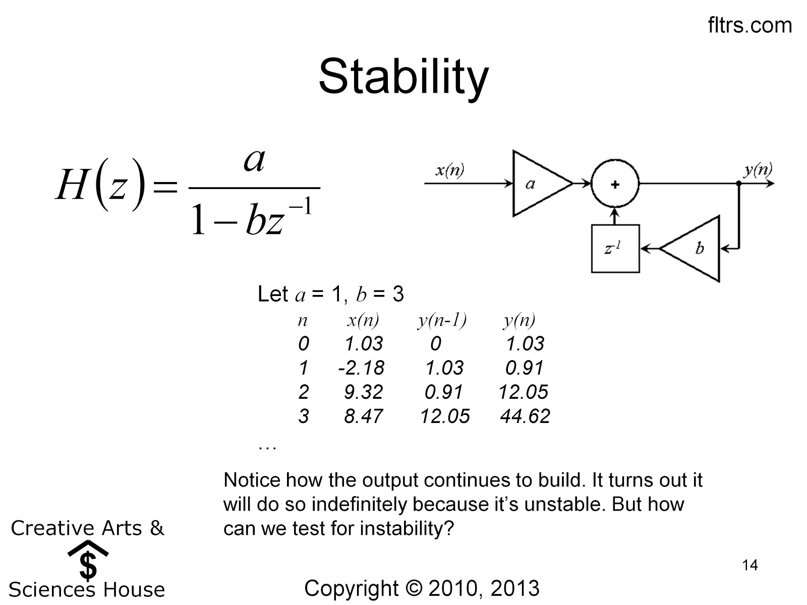
Now, we cannot tell from the output data above that the system is unstable, though we might be suspicious. But we can actually tell for sure even without computing the outputs, as we'll show below.

In our math unit we talked about the roots of polynomials. Transfer functions have (in general), both a numerator polynomial (upper portion) and a denominator polynomial (lower portion). 

We call the roots of the numerator polynomial zeros of the system, and the roots of the denominator polynomial poles.

System theory tells us that a stable system must have poles with magnitudes strictly less than 1. Another way of saying this is that they much lie within the "unit circle," a circle in the complex plane with radius 1.

Our pole is 3, which is definitely greater than 1. As we suspected earlier, this system is unstable!

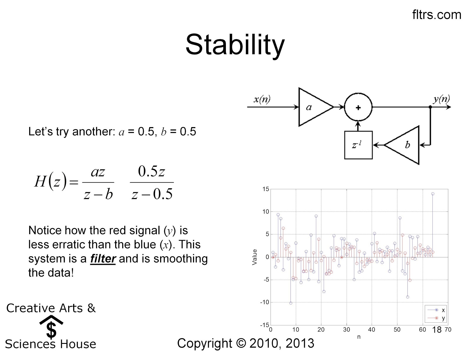
Let's try the case below:

We see above that the new pole is within the unit circle, so this is stable. But what does this system do?

We generated a random noise signal (blue) and passed it through this system. The output (red) is a little smoother. It turns out that we have created a simple filter.

Now let's try looking at this sort of thing in the opposite direction.

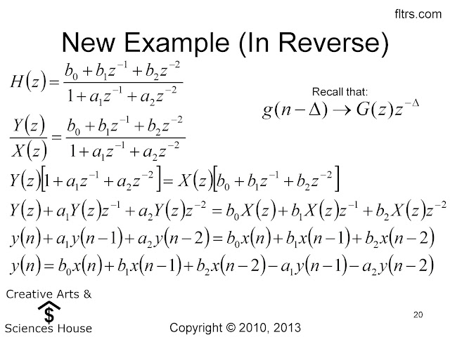
We can apply our z-transform relationship in reverse this time. Follow along.

Does it make sense? We've gone from a transfer function to a system equation. Now we can go from that to a block diagram. Note that there is more than one block diagram that will implement this equation, but that they are all mathematically the same (though might have some practical differences). Here we have drawn the "Direct Form I" diagram to implement this equation. More about that in a later unit.

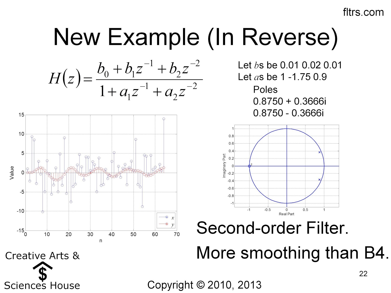
What does this system do? Well, again its coefficients make a difference as to its exact functionality. But again it's a filter (lowpass in fact) that smooths out the input even more than did our previous filter.

Notice that the poles are now complex, but that they do reside within the unit circle. The system is stable.

Digital Filter University - Course II: The Math

As you might have already noticed, I love everything about digital filters. And I love math too, especially filter math. It's a great myth that engineers are good at math. Most of us aren't. Even the math we studied we forget. So, if you are an engineer, don't feel bad about looking this over as a refresher. If you're not an engineer or an otherwise mathy person, let me see if I can give you adequate background for use in digital filters. If there is ever anything you cannot follow, let me know and I'll help. Your questions will help others, so fire away.

I once took a math class where the professor said he would write on the board all the things we needed to know from our previous math courses. He wrote a y on the board, and then stood in front of what he was writing so we couldn't see. I imagined that he was writing something like y = mx+b, which is the equation for a line, and an important element of math. But, when he finished and moved aside, he had written "everything!" 

Well, never fear. I would never do such a thing to you, would I? Actually, there are only a few mathematical concepts needed for digital filtering. Much less than you would expect. I'll show you:

Let's start by talking about the real numbers. You already know all this; but in case you are a little rusty (no pun) on the details, let's review. Numbers can be plotted on a number line or on what we can an x-y axis, as shown at right below. When the numbers are in (x, y) pairs, we find the location on the x-axis, and then move up (or down, if the y value is negative) to the location on the y-axis. Make sure you now how to plot the points plotted on the axis below.

It's also useful to recall a few properties of real numbers. A number multiplied by itself is the number squared. However, if we take the square root of a number, we are looking for a number that, when squared, will equal the original number. Remember that a negative number times a negative number gives a positive result. So the square root of a number can be either positive or negative and, when squared, the original number will return like magic.

If we multiply a number by itself three times, we get the cube. The cube root, however, has to have the same sign as the original number, because three negatives multiplied return a negative. Can you follow all the stuff on this next chart? 

I suppose "imaginary numbers" is a weird name since these numbers are actually "real" in the sense that they do exist. But we already used up the name real on the previous type of numbers, so these numbers got stuck with a name that makes you think you don't need to worry about them, as in the case of the imaginary monsters who used to live in your closet or under your bed. Not so. Our imaginary friends of the numerical variety actually make digital filters tick. So quit drowsing off and pay a little attention for once, would ya!?

We, appropriately, in my view, use the letter i to indicate imaginary numbers. Some'a you electrical engineers may also be used to using j. That practice was started to avoid confusion with the i that's used for current. There never would have been such a problem had something reasonable been used for current in the first place... But, though I do have a small stack of electrical engineering degrees, I'm a digital filter guy. I don't deal much with current except when I go fishing. And I haven't been fishing in at least a decade. So, forgive me if I use i. I prefer it.

Now, i is actually defined as the square root of negative 1. You may have heard that the square root of a negative number is not defined or doesn't exist. Just one of many lies you've been told throughout your life. Get over it.

Given that definition for i, it's clear that it's square has to be -1. It's cube is actually -i since the cube is the square times i. Makes sense, right?

Look over the notes below and make sure you follow. Ask if you have a question.

Now, whenever an imaginary number gets together with a real number, the result is a complex number. This is another unfortunate name, since complex numbers really aren't all that complex. It might have been nice had they been called composite numbers or something instead.

One key thing to remember about complex numbers is that the real and imaginary parts must be kept separate. Notice below how we have a number 2 + 3i. That is the simplest form for that number.

This is what happens when a real number is multiplied by an imaginary number: 4 x 5i = 20i. See what happened there? 

What about when two imaginary numbers are multiplied? 4i x 5i = -20 because the two is combine to make i squared, which is -1. Slick ain't it?

Look over the chart below to make sure you can follow both the plotting and the arithmetic. Recall the FOIL rule from algebra: when we multiply any pair of numbers, like x + y, or 2 + 3i with another pair, we multiply the First elements with each other, then the Outside elements, then the Inside elements, and then the Last elements. Work through to make sure you get the same result.

I'll wait while you work out the examples below. Let me know when you've finished.

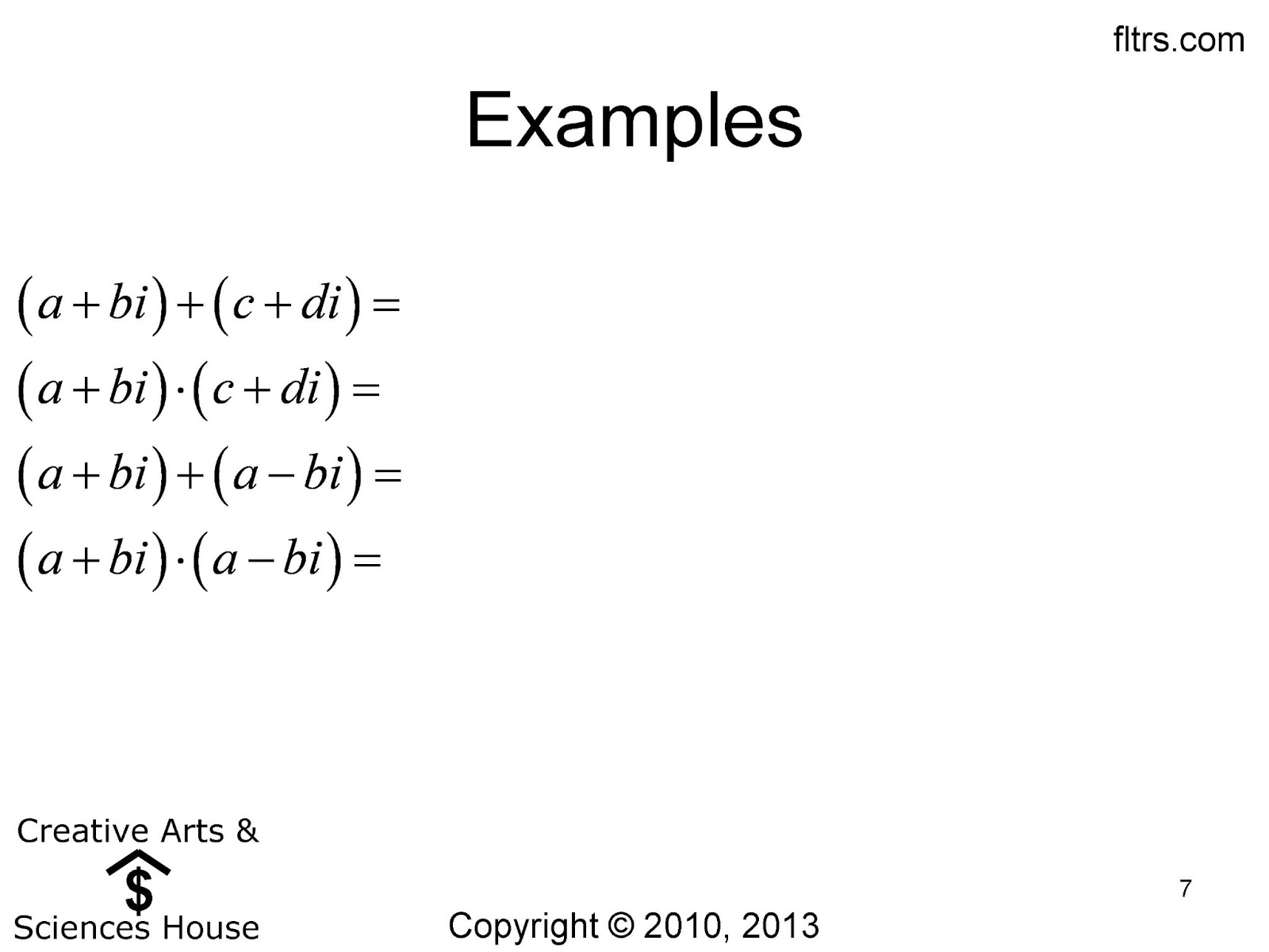
How'd that go? Did you get them right? Here's what I got:

Now that we're experts on that, it's time to move on to a new topic: polynomials. If you are familiar with the filter song, you know that polynomials are highly revered in the filter world.

Although polynomials can be written in terms of other variables, the ones below are polynomials in x. In the first one, we have x, or x^1 if you prefer. So this is a first-order polynomial. Notice how the order is the highest power of x in the polynomial. 

The roots of polynomials are those values of x that make the polynomial go to 0. The first order case is simple, as seen below. Check it, to make sure it's correct.

Some second order polynomials are easy to factor, as you see in the next chart. If x + 3 is a factor of the polynomial, and we plug in -3 for x, that factor goes to 0 right? And, of course, if we multiply that 0 by the other factor, the result is still 0. So we see that we can simply get the roots from the factors.

Try your hand at factoring these.

Here's what I got for the first three. But the last one doesn't factor simply.

There's nothing that says polynomials have to have simple, integer roots. In fact, they don't even have to be real. So, when something doesn't factor simply, or even if it does, we can use the quadratic equation to factor 2nd order polynomials.

Now, follow along as I plug the roots back in to make sure they're correct.



As Peter Gabriel would say, "don't give up." One more slide to go (for this example, anyway).

This next one turns out to be real, but still irrational. That is, it's not a simple integer number, but it has no imaginary part. Follow along.



There is something magic about 2nd order polynomials. As we've said, their roots are not always complex. In fact, the only way they can be complex is if they occur in what we call complex conjugate pairs. This is explained below. Awesome, ain't it?

Unfortunately, there is no such simple formula for factoring higher order polynomials. But, at least there are dozens of ways - websites, calculators, computer software - to get the job done. Note that we usually need decent precision for filter work, and some websites that I've tried didn't have it. Look for something similar to the number of decimal places we have below.

Some people get concerned when they look at filter formulas because they notice a tangent or a cosine here and there. Fortunately for both you and for me, we don't have to know (or remember) all those trigonometric identities. Don't get me wrong, I like trig. But that doesn't mean I remember them either.

Generally speaking, for filter work, we really only need to evaluate the trigonometric functions. When I was a kid this meant looking in a book for a table of values, and then interpolating the table to get the answer. But don't worry, I'm not a kid anymore. As with factoring higher order polynomials, evaluating trigonometric functions is now the domain of software. Just plug in the input (argument), and get the output. That's all there is to it. These days a $10 calculator will even do it, as will the one on your computer (if you select scientific calculator mode).

The inverse of the tangent function is called the inverse tangent or the arctangent. Similarly with the other trig functions. Exactly what this means is shown below.

I once developed an algorithm that was full of trigonometric functions. In an effort to prove that I am not a unidimensional human being, I named it Death Comes for the Arctangent (after a similarly named Willa Cather novel). But now I really am off on a tangent.

Let's refresh our memories about degrees and radians below. Got it?

Now, of course we can plot the points on an axis, as we have discussed previously. But sometimes we need to know the angle from the positive x-axis to the line segement between the origin and these points, as shown in the chart below?

As you may have guessed, the answer involves the arctangent. But, did you ever hear about the quadrants of two-dimensional plots? We call the upper right one quadrant I, and then number them counter clockwise from there, I - IV. Unfortunately the regular arctangent doesn't understand about quadrants. It gives you part of the information you need, but then you sometimes have to compensate it to get the quadrant correct, as shown below.

An alternative to this is something called the two input arctangent or atan2. (Some math software abbreviates arctangent as atan, and the two input version as atan2.) This version does know about quadrants and can, therefore, give you the angle you need without compensation.



Now, this might seem like a big shift from where we were, but the final note for this unit is about polar coordinates. When we plot x and y values, we are using rectangular or cartesian coordinates. (Named for Rene Descartes who thought, therefore he was.)

But we can also specify a point ono the grid by what we call polar coordinates, which tell us the angle, as we have already discussed, and the magnitude, or length of the line segement from the origin. Note that either set of coordinates can describe the same point. And, we can convert back and forth between them, as described below.

The exponetial of itheta might look a little unusual. But just think of this notation as describing the angle to the point. (Or study it more. It's actually quite fascinating.)











Now, if you ever encounter a polar bear, you can quicky convert him into a cartesian bear. Then, if you don't think about him, maybe he'll cease to exist? If you try it, let me know how it comes out.

We'll introduce a few more mathematical concepts as needed in the course of the remaining lectures. But generally speaking, if you can get through this, you've got the foundation you need to deal with digital filters. If you can't get through this, don't give up. Let me know and I will help you. You can do it, for sure.